More data than you know what to do with
It’s increasingly common for information workers to come in contact with unfamiliar datasets. Governments around the world are releasing more and bigger datasets. Corporations are collecting and releasing more data than ever, often in XML or another format easily convertible to XML. This trend, while welcomed by many, poses questions about how to come to understand large XML datasets.
In general, bulk analysis of large datasets gets done through an ad-hoc assortment of machine learning techniques. Few of these, however, are specifically targeted at the unique aspects of the XML data model, as examined in this paper.
One tool in particular that has come into widespread use for analyzing datasets is R, which has available a set of XML libraries R Language; Package 'XML'. However, while R is often useful for initial exploration, it lacks an upgrade path into an operational data store such as an XML database, and the XML capabilities provided are DOM and XPath-centric, which are less suited to bulk analysis.
The most common approach used by databases to deal with searching and navigating through large datasets is an index, trading space for time. Once an index is set up and occupying additional disk and/or memory space, certain kinds of queries run significantly faster.
With an unknown dataset, though, this presents a chicken-and-egg problem. Many database systems assume the availability of indexes to perform navigational functions such as faceted search. Without such features, it’s more difficult to get to know the data. And if the structure of the data is unknown, how can one create the necessary indexes in the first place?
One answer is that indexes should be arranged based on queries rather than data. This is a valid approach, although not of much help in the case of bootstrapping a truly unknown dataset.
Another approach, one explored in the remainder of this paper, is to rely on statistical sampling approaches rather than indexes. This presents tradeoffs in terms of size, speed, and accuracy. At the same time, it offers benefits:
|
Rapid start |
The ability to run queries immediately, without prior configuration. |
|
Productivity |
The ability to run queries before or during a lengthy indexing operation. |
|
Exploration |
An aid to identifying areas in the dataset that might requires some amount of cleanup before applying indexing. |
|
Cross-platform development |
None of the techniques here depend on proprietary index structures. |
|
Performance baselining |
These techniques can be used as a measuring stick to compare the size and speed tradeoffs of various index configurations. |
Though the techniques shown here are universally applicable, for convenience, code samples in this paper are based on an early access release of MarkLogic 6 MarkLogic docs.
Random Sampling
A common approach to characterizing a large population involves taking a random sample. A simple XQuery expression
fn:collection()[1]takes advantage of the implementation detail that many databases define document order across the entire database in an arbitrary order so that the "first" document is essentially a random choice. One common manual approach is to "eyeball" the first such document, and maybe a few others, to get an intuitive feel for the kinds of data and structures at hand. This approach has obvious scaling difficulties.
For larger samples, greater automation is needed for the analysis. We can define a process producing a sample of size N to be considered random if any particular collection of documents is equally likely to turn up as any other same-sized collection of documents. Randomness of a sample is important, because a non-random sample will lead to systematic errors not accounted for in statistical measures of probability.
Within a random sample it is possible to examine characteristics of the sample and make statistical inferences about the overall population. The more documents in the sample, the better the approximation. When the overall population is small, it is possible to sample most or even all of the documents. But with large collections of documents, the proportion of documents contained in a reasonably-sized sample will be very small. When dealing with a dataset of this size, certain simplifying assumptions become possible, as outlined in later sections of this paper.
Users of search interfaces have become accustomed to approximations, for example, a web search engine may report something like “Page 2 of about 415,000,000 results”, but as users go deeper into the result set, the estimated number tends to converge on some actual value. Users have accepted this behavior, though it is less commonly used in finer-grained navigational situations. For example, if a sidebar on a retail site says, “New in last 90 days (328)”, quite often one will find that exactly 328 items will be available by clicking through all the pages of results.
This difference in user expectations can be exploited. In particular, in the case of first contact with a new XML dataset, exact results are far less important than overall trends and correlations, which makes a sampling approach ideal.
Sample size end error
Statistical estimates by definition are not completely reliable. For example, it's possible (though breathtakingly unlikely) that a random sample of 100 documents would happen to contain all 100 unusual instances out of database of a million documents. A surer bet, though, would be none of the unusual documents would turn up in a sample of 100. One measure of an estimate's reliability, called a confidence interval is related to a chosen probability range. To put it another way, if the random experiment were repeated many times whereby it was found that 95.4% of the calculated confidence intervals included the true value, one could say that 95.4% was the confidence interval. (Note, however, that when speaking about a single experiment, the estimated range either contains the true value or it doesn't and one would need more complicated Bayesian techniques to delve deeper.)
For a large population, it is convenient to use a confidence interval of 95.4%, which encompasses values two standard deviations from the mean in either direction and makes the math come out easier later on. At that confidence level, and assuming a large overall population relative to the sample size, the maximum margin of error is simply (continuing to use XQuery notation)
1 div math:sqrt($sample-size)
although in particular cases, the observed error can
be somewhat less.
For example, a sample size of 1000, likely to be conveniently held in memory, the maximum margin of error comes out to about 3.16%, which is good enough for many purposes.
A key weakness in sampling is that rare values are likely to be missed. A doctype that appears only 100 times out of a million is unlikely to show up in a sample of 100 documents, and on rare occasions when it does show up exactly once, straightforward extrapolation would infer that it occurs in 1% of all documents, a gross overestimation.
Performance
The approaches in this paper assume that an entire sample of documents can comfortably fit into main memory. To fulfill a random-sampling query without indexes, each document needs to be read from disk. Therefore, overall the performance of the query will be roughly linear in the sample size, plus time for local processing. Details will vary depending on the database system, but in general there will be some amount of data locality making for shorter document-to-document disk seeks. A back-of-the-envelope estimate is about 1 second per 200 documents in the sample, ignoring the prospect of documents cached in memory, perhaps somewhat higher with high-performance disks such as SSD or RAID configurations that stripe data across multiple disks.[1].
Dipping a toe into the database
Getting familiar with an XML dataset requires a combination of automated and hands-on approaches. While writing this paper, I had on hand a dataset of over 5 million documents, crawled from an assortment of public social media sources, of which I knew very little in advance.
The first-document-in-the-collection approach mentioned above yields this [2]:
<sl:streamlet
xmlns:sl="http://example.com/ns/social-media/streamlet">
  <sl:vid>13067505336836346999</sl:vid>
  <sl:tweet>#Jerusalem #News 'Iran cuts funding for
  Hamas due to Syria unrest'
  http://t.co/ARRqabU</sl:tweet>
</sl:streamlet>
The choice of the "first" document, is, of course, completely arbitrary. The second document has something completely different:
<person:person
xmlns:person="http://example.com/ns/social-media/person">
  <person:id>8999631448253261463</person:id>
  <person:follower-count>0</person:follower-count>
  <person:influence>0</person:influence>
  <person:name>Borana Mukesh</person:name>
  ...
</person:person>
There's only so much one can learn from picking through individual documents.
The following XQuery 3.0 XQuery 3.0 code demonstrates this approach by examining a sample of documents in order to extract potentially interesting features, which a human operator can use to make decisions about where to dive deeper. The code assembles the following:
-
Root elements
-
Commonly-occurring elements
-
Commonly-occurring namespaces
-
Elements that tend to have a lot (or a little) text content
-
Text nodes that look like dates
-
Text nodes that almost look like dates
-
Text nodes that look like numeric data, for example years
  let $dv := distinct-values#1
  let $n := ($sample-size, 1000)[1]
  let $xml-docs := spx:est-docs()
  let $text-docs := spx:est-text-docs()

  let $samp := spx:random-sample($n)
  let $cnames := $dv($samp/*/spx:name(.))
  let $all-ns := $dv($samp//namespace::*)
  let $leafe := $samp//*[empty(*)]
  let $leafetxt := $leafe[text()]
  let $leafe-long := $leafetxt
    [string-length(.) ge 10]
  let $leafe-short := $leafetxt
    [string-length(.) le 4]
  let $dates := $dv($leafe-long
    [. castable as xs:dateTime]/spx:name(.))
  let $near-dates := $dv($leafe-long
    [matches(local-name(.), '[Dd]ate')]
    [not(. castable as xs:dateTime)]/spx:name(.))
  let $all-years := $dv($leafe-short
    [matches(., "^(19|20)\d\d$")]/spx:name(.))
  let $all-smallnum := $dv($leafe-short
    [. castable as xs:double]/spx:name(.))
  let $epd := count($samp//*) div count($samp/*)
  return
    <spx:data-sketch
      xml-doc-count="{$xml-docs}"
      text-doc-count="{$text-docs}"
      binary-doc-count="{$binary-docs}"
      elements-per-doc="{$epd}">
      {$cnames!<spx:root-elem
        name="{.}"
        count="{spx:est-by-QName(spx:QName(.))}"/>
      }
      {$all-ns!<spx:ns-seen>{.}</spx:ns-seen>}
      {$dates!<spx:date>{.}</spx:date>}
      {$near-dates!<spx:almost-date>{.}</spx:almost-date>}
      {$all-years!<spx:year>{.}</spx:year>}
      {$all-smallnum!<spx:small-num>{.}</spx:small-num>}
    </spx:data-sketch>
This code and the following listings make use of the following helper functions which contain vendor-specific implementations, which are not important here (see the Code section later for details):
|
spx:est-docs() |
A function that quickly estimates the total number of documents in the database. |
|
spx:est-test-docs() |
A function that quickly estimates the total number of documents in the database that consist of a single text node. |
|
spx:random-sample() |
A function that returns a random sample of documents from the database. |
|
spx:name() |
Returns a Clark name of a given node. |
|
spx:formatq() |
Returns a Clark name from a given QName. |
|
spx:node-path() |
Returns an XPath expression that uniquely identifies a node. |
This code produced the following (with adjustments for line length):
<spx:data-sketch
xmlns:spx="http://dubinko.info/spelunx"
  xml-doc-count="5789128"
  text-doc-count="0"
  binary-doc-count="0"
  elements-per-doc="12.88" >
  <spx:root-elem name="{...}person" count="1248848"/>
  <spx:root-elem name="{...}media" count="2117625"/>
  <spx:root-elem name="{...}streamlet" count="1173545"/>
  <spx:root-elem name="{...}author" count="1248815"/>
  <spx:ns-seen>
    http://example.com/ns/social-media/person
  </spx:ns-seen>
  <spx:ns-seen>
    http://example.com/ns/social-media/media
  </spx:ns-seen>
  <spx:ns-seen>
    http://example.com/ns/social-media/streamlet
  </spx:ns-seen>
  <spx:ns-seen>
    http://example.com/ns/social-media/author
  </spx:ns-seen>
  <spx:ns-seen>
    http://www.w3.org/XML/1998/namespace
  </spx:ns-seen>
  <spx:date>{...}ingested</spx:date>
  <spx:date>{...}published</spx:date>
  <spx:date>{...}canonical</spx:date>
  <spx:date>{...}inserted</spx:date>
  <spx:small-num>{...}follower-count</spx:small-num>
  <spx:small-num>{...}influence</spx:small-num>
  <spx:small-num>{...}follower-count</spx:small-num>
</spx:data-sketch>
This dataset appears fairly homogeneous: only four different root element
QNames, were observed over 1,000 samples. Additionally, these documents
contain a number of elements that seem date-like, but would require some
cleanup in order to be represented in as the Schema datatype xs:dateTime.
For purposes of this paper, one particular element, influence,
as seen earlier, seems particularly
interesting. Is there a way to learn more about it?
Digging Deeper
It’s possible to perform similar kinds of analysis on specific nodes in the database. Given a starting node, the system of XPath axes provides a number of different ways in which to characterize that element’s use in a larger dataset. Some care must be taken to handle edge cases, assuming nothing in an unknown environment. The following code listing characterizes a given element node (named with a QName) along several important axes:
  let $dv := distinct-values#1
  let $n := ($sample-size, 1000)[1]
  let $samp := spx:random-sample($n)

  let $ocrs := $samp//*[node-name(.) eq $e]
  let $vals := data($ocrs)
  let $number-vals := $vals
    [. castable as xs:double]
  let $nv := $number-vals
  let $date-values := $vals
    [. castable as xs:dateTime]
  let $blank-vals := $vals[matches(., "^\s*$")]
  let $parents := $dv(
    $ocrs/node-name(..)!spx:formatq(.))
  let $children := $dv($ocrs/*!spx:name(.))
  let $attrs := $dv($ocrs/@*!spx:name(.))
  let $roots := $dv($ocrs/root()/*!spx:name(.))
  let $paths := $dv($ocrs/spx:node-path(.))
  return
    <spx:node-report
      estimate-count="{spx:est-by-QName($e)}"
      sample-count="{count($ocrs)}"
      number-count="{count($number-vals)}"
      date-count="{count($date-values)}"
      blank-count="{count($blank-vals)}">
      {$parents!<spx:parent>{.}</spx:parent>}
      {$roots!<spx:root>{.}</spx:root>}
      {$paths!<spx:path>{.}</spx:path>}
      <spx:min>{min($number-vals)}</spx:min>
      <spx:max>{max($number-vals)}</spx:max>
      {if (exists($vals)) then
      <spx:mean>
        {sum($nv) div count($nv)}
      </spx:mean>
      else ()
      }
    </spx:node-report>
These two techniques combine to provide a powerful tool for picking through an unknown dataset. First identify ‘interesting’ element nodes, then dig into each one to see how it is used in the data. While the sample documents are in memory, it is possible to infer datatype information, and for values that look numeric, to calculate the sample min, max, mean, median, standard deviation, and other useful statistics.
These techniques can be readily expanded to include statistics for other node types, notably attribute and processing-instruction nodes.
Free-form faceting
Index-backed approaches make it possible to produce a histogram of values, often called "facets", for example all the prices in a product database, arranged into buckets of values like 'less than $10' or '$10 to $50' and so on.
It’s possible to combine the concepts introduced thus far by breaking down a random
sample into faceted data.
With no advance knowledge of the range of values, it’s difficult to arrange values
into
reasonable buckets, but with some spelunking, as in the preceding section,
it’s possible to construct reasonable bucketing. Based on the exploration
from the preceding sections, the influence element looks
worth further investigation.
The following XQuery function plots out the values of a given element as xs:double values in specified ranges.
declare function spx:histogram(
  $e as xs:QName,
  $sample-size as  xs:unsignedInt?,
  $bounds as xs:double+
) {
  let $n := ($sample-size, 1000)[1]
  let $samp := spx:random-sample($n)
  let $full-population := spx:est-docs()
  let $multiplier := ($full-population div $n)
  let $ocrs := $samp//*[node-name(.) eq $e]
  let $vals := data($ocrs)
  let $number-vals := $vals
    [. castable as xs:double]!xs:double(.)
  let $bucket-tops := ($bounds, xs:float("INF"))
  for $bucket-top at $idx in $bucket-tops
  let $bucket-bottom :=
    if ($idx eq 1)
    then xs:float("-INF")
    else $bucket-tops[position() eq $idx - 1]
  let $samp-count := count($number-vals
    [. lt $bucket-top][. ge $bucket-bottom])
  let $p := $samp-count div $n
  let $moe := 1 div math:sqrt($sample-size)
  let $SE := math:sqrt(($p * (1 - $p)) div $n)
  let $est-count := $samp-count * $multiplier
  let $error := $SE * $full-population
  let $est-top := $est-count + $error
  let $est-bot := $est-count - $error
  return
    <histogram-value
      ge="{$bucket-bottom}"
      lt="{$bucket-top}"
      sample-count="{$samp-count}"
      est-count="{$est-count}"
      est-range="{$est-bot} to {$est-top}"
      error="{$error}"/>
};
This code accepts a particular QName referring to an element, a
sample size, and an ordered set of numeric bounds, and returns the
approximate count of values that occur in between each boundary. The first
bucket includes values down to -INF, and the last bucket
includes all values up to INF. Selecting values to partition
the values into order-of-magnitude buckets will give a broad first
approximation of the distribution.
For comparison, the following vendor-specific code, which requires a pre-existing in-memory index, resolves the exact counts of different values occurring in the database.
for $bucket in cts:element-value-ranges(
  QName("http://example.com/ns/social-media/person", "influence"),
  (1,10,100,1000), "empties")
return
    <histogram-value
        ge="{($bucket/cts:lower-bound, '-INF')[1]}"
        lt="{($bucket/cts:upper-bound, 'INF')[1]}"
        count="{cts:frequency($bucket)}"/>
The results of calling these function on the test database are given below in table format.
How wrong can you get?
As the book Statistics Hacks Statistics Hacks states,
Anytime you have used statistics to summarize observations, you’ve probably been wrong.
This technique is no exception.
As mentioned earlier, if we assume that the sample is of a small proportion of the overall population and is randomly selected, the maximum margin of error is a simple function of sample size. However, against particular values we can usually find a more accurate estimate.
To estimate the overall proportion, the standard error of the proportion must be computed, using the following formula.
math:sqrt(($p - $p * $p) div $sample-size )The maximum error, which occurs when the proportion is exactly 50%, is exactly half of the margin of error calculation earlier[3].
The following table illustrates the tradeoffs in accuracy, run-time, and necessity of a preconfigured index. The columns on the left represent histogram buckets of values of various ranges, while the rows across the top represent different sample sizes, or in the case of the final column, exact index resolution. The hardware under test consisted of a 2.4Ghz Dual-core 64-bit Intel machine with two 15k rpm disks in a RAID O configuration.
Table I
Comparison of run-time and accuracy
| estimate, n=10 | estimate, n=100 | estimate, n=1000 | estimate, n=10000 | exact index resolution | |
|---|---|---|---|---|---|
| values < 1 | 115,7825 | 810,477 | 897,314 | 782,111 | 807,284 |
| 1 <= values < 10 | 0 | 0 | 17,367 | 25,472 | 28,414 |
| 10 <= values < 100 | 578,912 | 115,782 | 208,408 | 164,990 | 161,734 |
| 100 <= values < 1000 | 578,912 | 347,347 | 219,986 | 208,408 | 204,298 |
| values >= 1000 | 0 | 0 | 28,945 | 36,471 | 47,070 |
| Run time | 0.35 sec | 0.48 sec | 1.9 sec | 19.4 sec | 0.19 sec |
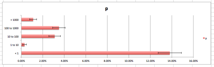
Unsurprisingly, at smaller sample sizes, it is probable that infequently-occurring data will be completely excluded from the random sample. Even the most frequently-occurring values, in this case the bucket of values less than one, occurs in less than 14% of the 5.7M documents. Given this, the accuracy of the random sampling technique, even at the lower sample counts, is more than enough to give a general impression of the distribution of the data values.
To visulaize this, it is possible to export these values into a desktop spreadsheet program and produce a graph, including error bars, as shown in the following figure.
Figure 1: Graphical representation of data distribution (by percentage)
Conclusion
The techniques shown in the paper offer a useful framework within which to make the initial foray into an unknown XML dataset. Starting with an automated run-down of high-level features in the dataset, particular QNames chosen by the user can be drilled down into deeper analysis. The dataset can even be summarized through histogram facets, much like those available to significantly more resource-intensive indexed databases.
The techniques shown here do not rely on proprietary features and are applicable to a wide range of available XQuery processors.
The book How to Lie with Statistics How to Lie with Statistics concludes with advice on how to be properly skeptical of statistics, and the guidelines apply to the techniques in this paper as much as in any other area.
|
What's missing? |
Be on the lookout for areas where summarization may be obscuring important facts. |
|
Did somebody change the subject? |
Beware of an unfounded jump from raw figures to conclusions. |
|
Does it make sense? |
Any results that come from these techniques need to be eyeballed. Anything that seems wildly out of proportion needs to be more closely examined. |
With those caveats, the techniques in this paper can provide a useful lever by which to pry open a large, unkonwn XML data set.
Code availability
The code samples mentioned in this paper are in available in a project named Spelunx available at GitHub Spelunx.
Further topics to explore
-
Correlation and co-existence between given nodes
-
Multi-dimensional sampling, as in geographic data
-
Searching for correlated latitude and longitude pairs
-
Hypothesis testing and type I vs type II errors
-
Markov chain analysis for element and attribute containership
-
Comparison and contrast with machine learning techniques
-
Exploring the availability of random-sampling extension functions from different database vendors
-
Ways to summarize mixed content
References
[R Language; Package 'XML'] Duncan Temple Lang (editor), Package 'XML', version 3.9-4
[online]. [cited 13th July, 2012]. http://cran.r-project.org/web/packages/XML/XML.pdf
[XQuery 3.0] Jonathan Robie, Don Chamberlin, Michael Dyck, and John Snelson (editors), XQuery 3.0: An XML Query Language
[online]. [cited 13th July 2012]. http://www.w3.org/TR/2011/WD-xquery-30-20111213/
[MarkLogic docs] MarkLogic Corporation, MarkLogic Server Search Developer's Guide
[online]. © 2012 [cited 13th July 2012]. http://developer.marklogic.com/pubs/5.0/books/search-dev-guide.pdf
[Clark notation] James Clark, XML Namespaces
[online]. [cited 13th July, 2012]. James describes "universal names written as a
URI in curly brackets followed by the local name" which have proved to be a useful
construction in more contexts than explaining namespaces. http://www.jclark.com/xml/xmlns.htm
[Statistics Hacks] Bruce Frey, Statistics Hacks: Tips & Tools for Measuring the World and Beating the Odds
(O'Reilly Media, 2006). Despite the name, includes a great deal of basic information
on statistics and the math behind it.
[How to Lie with Statistics] Darrell Huff, How to Lie with Statistics
(W. W. Norton & Company, 1993 reprint). To appreciate the power of statistics, you
must understand how it can be used as a weapon.
[Spelunx] Micah Dubinko, Spelunx
open source project [online] https://github.com/mdubinko/spelunx
[1] In general, document-level caching provides little benefit for random-sampling based approaches, as a different random set of documents gets selected on each run of the experiment.
[2] Namespace URIs have been anonymized.
[3] Half because margin of error already accounts for error in the plus or minus direction, i.e. a diameter, while standard error or the proportion does not, i.e. a radius.