Introduction
Practitioners of descriptive markup rely on the ability of markup in a document to convey information; earlier work has attempted to characterize the nature of that information and describe ways to make it manifest in ways beyond what is done by conventional processing of SGML, XML, and similar systems.[1] Among the methods so far suggested is to capture the information carried by the markup of the document in symbolic logic. It is possible in principle to enumerate the crucial inferences licensed by the markup in a document; these sentences, together with all the other sentences that can be inferred from them, are held to constitute the set of inferences licensed by the markup (which in turn is held by some to constitute the meaning of the markup).
We offer here an application of that idea to the problem of document comparison. Given the sets of inferences licensed by the markup in two documents, we suggest a method for determining whether the markup in the two documents is semantically equivalent, semantically compatible (but richer in one than the other), or contradictory.
One consequence of this is that the information in documents can usefully be taken to form a lattice, which can in turn be used to illustrate the relation among documents.
Document comparison
Relations among documents
We claim that with respect to the information carried by the markup in any two documents D1 and D2, exactly one of the following states of affairs will apply:
-
D1 and D2 are equivalent: all of the information in D1 is present in D2 and vice versa.
-
D1 subsumes or is an abstraction of D2: all of the information in D1 is present in D2, but the reverse is not true. Equivalently, we say that D2 is a refinement of D1.
-
D2 subsumes D1.
-
Neither D1 nor D2 subsumes the other, but they are logically consistent with each other.
-
D1 and D2 contradict each other.
An algorithm for document comparisons
To compare two documents D1 and D2, we first enumerate a set of key inferences from the markup for each document. Let us call these two sets S1 and S2. These take the form of sentences in some suitable form of symbolic logic. (In the example below, we use a more or less standard first-order predicate calculus; in demonstrating that the comparisons can be implemented in software, we also use the syntaxes of Prolog and Alloy.)
Note that we do not ask for an enumeration of all the
inferences licensed by the markup in either document; that set
is by definition closed under inference, and by all conventional
accounts will be infinite. By an enumeration of key
inferences
we mean some finite set of sentences inferred
from the document, which suffice to allow the inference of all
the others (sometimes called a basis for
the infinite set of inferences). We will refer to the closure
of S1 under logical
inference as *S1, and
the closure of S2
under inference will be
*S2.
In the simple case, S1 and S2 will use the same predicates, assume the existence of the same individuals, and use the same names for the individuals in the universe of discourse. Then establishing the informational equivalence of the two documents is simply a case of checking that every sentence in S1 is present in S2, and vice versa. The subsumption relation can similarly be established by checking for a subset relation between S1 and S2.
In the general case, however, none of these will be true:
S1 and
S2 may use different
predicates; they may assume the existence of different
individuals in the universe of discourse; even when they
assume the same
predicates or individuals, they
may use different names for them. A prerequisite for
comparing the sets
S1 and
S2 in practice is
thus the preparation of rules of inference that allow
statements in the vocabulary of
S1 to be inferred
from statements in the vocabulary of
S2, and vice-versa.
We will call these the translation inference
rules, since their goal is to translate information
from one vocabulary to another. Some translation inference
rules map from S1 to
S2: they allow us to
infer statements in the vocabulary of
S2, given other
statements in the vocabulary of
S1. We refer to
these as S1 →
S2; we refer to the
translation inference rules mapping in the other direction as
S2 →
S1.
Note that in what follows we silently assume that the translation inference rules S1 → S2 and S2 → S1 are given, and are included in the closures *S1 and *S2, along with other general world knowledge.
In this more general situation, we can establish the equivalence of D1 and D2 by checking that every sentence in S1 is present in, or follows from, S2, and vice versa. Subsumption, consistency, and inconsistency relations can similarly be established on the basis of logical implication.
We provide an algorithm for determining which state of affairs applies between documents D1 and D2:
-
From the set S1 and the translation rules S1 → S2, we attempt to infer each sentence in S2.
If we succeed for all sentences in S2, then S2 is contained within the logical closure of S1 (i.e. S2 ⊆ *S1, and by definition also *S2 ⊆ *S1). Less formally: all of the information in S2 is present in S1 (and similarly for D1 and D2).
If we succeed for some but not all sentences in S2, then some but not all of the information in S2 (and D2) is present in S1 (D1).
-
Conversely, from the set S2 and the translation rules S2 → S1, we attempt to infer each sentence in S1. (Or, more formally, we test whether *S1 ⊆ *S2.)
-
From the set S1 and the translation rules S1 → S2, we attempt to infer the negation of each sentence in S2.
If we succeed for any sentence in S2, then S1 and S2 contradict each other (as do D1 and D2).
If we fail for all sentences in S2, then S1 (and D1) are compatible (logically consistent) with S2 (D2).
-
Again, we perform the same task in the other direction, seeking to infer negations of sentences in S2 from the set S1 and the translation rules S1 → S2.
The relation of the documents' information content (as given by the markup) is determined by the results of this exercise.
-
D1 subsumes D2 if and only if each sentence in S1 can be inferred from S2 and S2 → S1.
-
D2 subsumes D1 if and only if each sentence in S2 can be inferred from S1 and S1 → S2.
-
D1 and D2 are equivalent if and only if D1 subsumes D2 and D2 subsumes D1.
-
D1 and D2 contradict each other if and only if ¬s1 follows, for some sentence s1 in S1, from S2 and S2 → S1, or ¬s2 follows, for some sentence s2 in S2, from S1 and S1 → S2.
-
D1 and D2 are compatible (logically consistent) with each other if and only if neither contradicts the other.
That is, the relation between documents D1 and D2 is determined by the subset/superset relations between *S1 and *S2.
The document lattice
The subset/superset relations among sets of inferences licenced by documents constitute a partial order over all documents. It is a consequence of this fact that the universe of documents forms a lattice, in the mathematical sense of the term.
A simple lattice formed by the subset relation over
the subsets of the {a, b, c} is:
Figure 1 Figure 2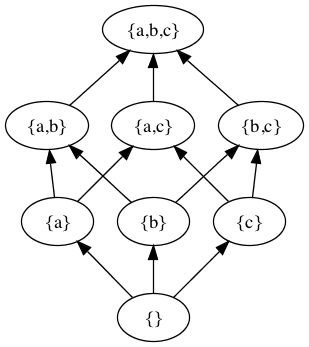
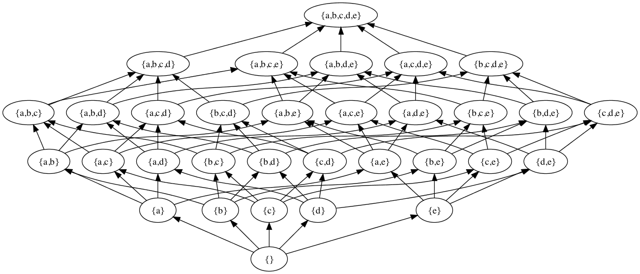
Any two points a and b in a lattice (and thus any two
documents in a lattice of documents) have both a greatest
lower bound (a point c in the lattice such that c ≤
a and c ≤ b, and x ≤ c for all x such that
x ≤ c and x ≤ b) and a greatest lower bound,
known in lattice contexts respectively as the
meet and the join of a and b.
Figure 3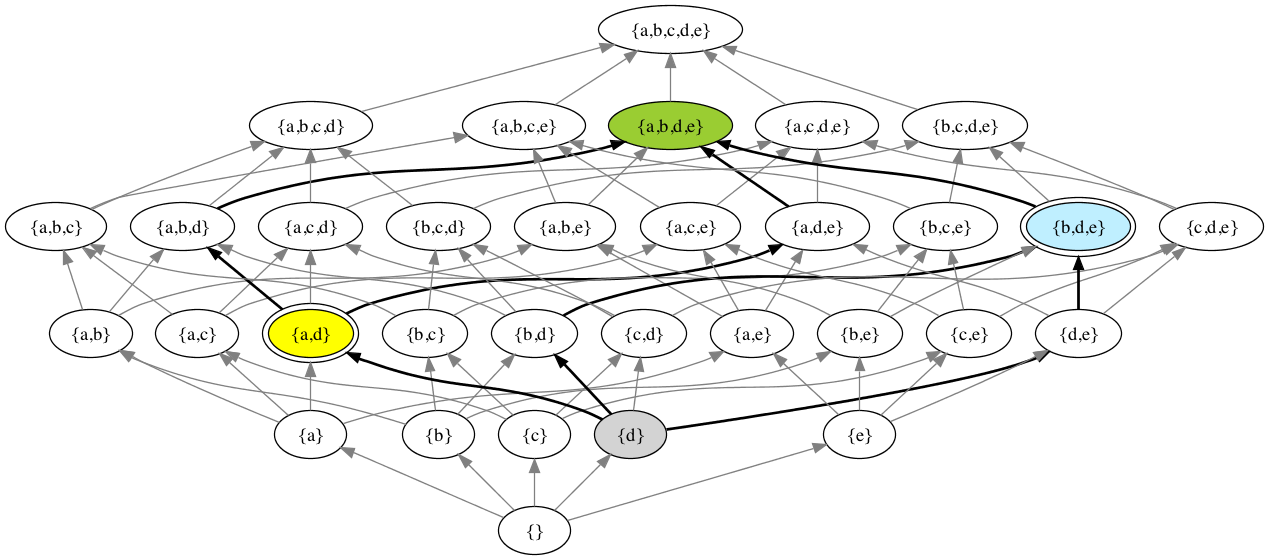
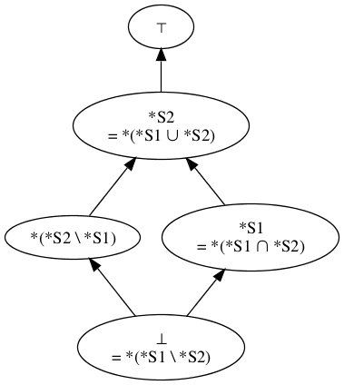
Since the set of documents is infinite, so is the universal document lattice (as we will call the lattice formed from the sets of sentences entailed by documents); we will not attempt to provide an image of this infinite lattice. Instead, we will illustrate document lattices by considering the lattice formed by the sets *S1, *S2, *(S1 ∪ S2), *(S1 ∩ S2), *(S1 \ S2), *(S2 \ S1), and the top and bottom nodes (⊤ and ⊥) of the universal document lattice.[2] Note that all illustrations assume that neither D1 nor D2 is self-contradictory (so neither *S1 nor *S2 is equal to ⊤) and that neither is vacuous (so neither *S1 nor *S2 is equal to ⊥).
Every document is represented by a point in the lattice. If and only if two documents D1 and D2 are equivalent, then D1 and D2 map to the same point in the lattice. If D1 subsumes D2 but the two documents are not equivalent, then D1 is below D2 in the lattice. Informally: we can reach D1 from D2 by going down in the graph (or D2 from D1 by climbing). If neither D1 nor D2 subsumes the other, then neither is above or below the other in the lattice.
For the document lattice (based as it is upon the subset relation), the meet of two documents D1 and D2 is represented by the set *S1 ∩ *S2, their join by *S1 ∪ *S2. (In the figure, the nodes a and b are colored yellow and blue; their meet is colored gray, their joint is colored green. As the bold arrows show, there may be more than one path connecting a node to its meet or its join with another node, but the meet and join are nevertheless each guaranteed unique.)
We have the following relations in the lattice for the various possible relations of D1 and D2, which we illustrate on the finite lattice described earlier:
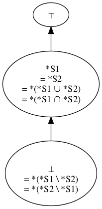
-
If D1 and D2 are equivalent, then they map to the same point in the lattice (as do their union and intersection).
Figure 4
-
If D1 subsumes D2 but they are not equivalent, then D1 is below D2 in the lattice and can be reached by a sequence of downward arcs.
Figure 5
-
If D2 subsumes D1 but they are not equivalent, then the reverse is true.
-
If D1 and D2 contradict each other, then their join is the topmost point in the lattice (the set of all possible sentences).[3]
Figure 6

-
If neither D1 nor D2 subsumes the other, but they are logically consistent with each other, then they have a join somewhere other than the top of the lattice.
Figure 7

Most of what has been said so far is a straightforward account of the relation of arbitrary sets of sentences in a logical notation, when the sets are closed under logical inference. It is not uniquely true of sets of sentences derived from the markup in documents. Readers thus may well be asking themselves where some application to document processing comes in.
The document lattice we have described makes explicit some facts about information in documents that is obvious to markup practitioners (but often disappointingly non-obvious to clients and novices). The kinds of translation processes referred to as up-translations and down-translations correspond directly to relations in the lattice: an up-translation involves mapping from some document D1 to another document D2 above D2 on the lattice, a down translation similarly involves moving downwards in the lattice.
If our task is to translate from document D1 in one markup vocabulary (say, Docbook) into some document D2 in another vocabulary (say, XHTML) by fully automatic means (e.g. an XSLT stylesheet), then either D2 must subsume D1, or our task is impossible: fully automatic transforms can in principle map only from one document into another document reachable by zero or more downward steps. (D2 is reachable in zero downward steps if it is logically equivalent to D1; this is possible in principle but often quite difficult in practice.)
If a conversion from one vocabulary to another is intended to have no information loss, then the requiremet is that for any D1 in the source vocabulary, the conversion produce a D2 which occupies the same point in the lattice.
Example
A simple example may help to illustrate the operation of the algorithm we have given above.
High-level description
Consider the following simple table:
Figure 8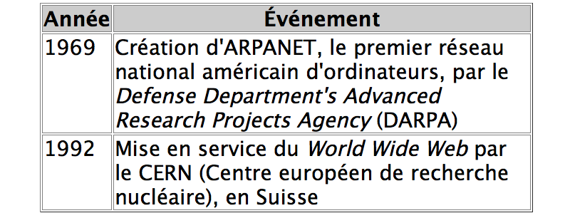
Let us imagine that we have two versions of this table, each in a different markup language with a possibly different table model, and we wish to know whether the table markup in the two documents is equivalent, or at least logically consistent.
One table, let us suppose, is tagged in XHTML:
    <table border="1">
      <tr>
        <th>Année</th>
        <th>Événement</th>
      </tr>
      <tr>
        <td>1969</td>
        <td>Création d'ARPANET, le premier réseau
        national américain d'ordinateurs, par le
        <em>Defense Department's Advanced
        Research Projects Agency</em> (DARPA)</td>
      </tr>
      <tr>
        <td>1992</td>
        <td>Mise en service du <em>World Wide Web</em>
        par le CERN (Centre européen de recherche
        nucléaire), en Suisse</td>
      </tr>
    </table>
The other table, intended to be equivalent, is tagged using the SGML Open exchange subset of the CALS table model [Bingham 1995], [Severson and Bingham 1995].
<table colsep="1" rowsep="1">
  <tgroup cols="2">
    <colspec colnum="1" colname="annee" colwidth="1*"/>
    <colspec colnum="2" colname="evenement" colwidth="4*"/>
   <tbody>
      <row>
        <entry>Année</entry>
        <entry>Événement</entry>
      </row>
      <row>
        <entry colname="evenement">Création d'ARPANET,
        le prémier réseau américain
        d'ordinateurs, par le Defense Department's
        Advanced Research
        Projects Agency (DARPA)</entry>
        <entry colname="annee">1969</entry>
      </row>
      <row>
        <entry colname="annee">1992</entry>
        <entry>Mise en service du World Wide Web
          par le CERN
          (Centre européen de recherche nucléaire),
          en Suisse</entry>
      </row>
    </tbody>
  </tgroup>
</table>
In first-order predicate calculus
From each marked up table we derive a set of sentences.[4]
Set S1
In more or less conventional first-order predicate calculus notation,[5] the first set of inferences is as follows.[6]
Table T is 3 by 2. In consequence, cell (3, 2) exists in table T, but cells (4, 1) and (1, 3) do not.)
-
table_dimensions(T, 3, 2)
-
cell(T, 3, 2) ∧ ¬cell(T, 4, 1) and ¬cell(T, 1, 3)
The two heading cells in row 1, columns 1 and 2, are identified as headings.
-
isTableHeader(T, 1, 1)
-
isTableHeader(T, 1, 2)
Next, the contents of the various cells are given.
-
tableCellContent(T, 1, 1, "Année")
-
tableCellContent(T, 1, 2, "Événement")
-
tableCellContent(T, 2, 1, "1969")
-
tableCellContent(T, 2, 2, "Création d'ARPANET...")
-
tableCellContent(T, 3, 1, "1992")
-
tableCellContent(T, 3, 2, "Mise en service du...")
The table has some styling information, given in CSS and not shown above: the table width is 80% of its parent element's width, and it has a 10% left margin.
-
tableWidth(T, "80%")
-
tableMarginLeft(T, "10%")
#CCCCCC, and all cells
are vertically aligned to the top of the cell.
-
(∀ x ∈ ℕ, y ∈ ℕ)[isTableHeader(T, x, y) ⇒ tableCellBackgroundColor(T, x, y, "#CCCCCC")]
-
(∀ x ∈ ℕ, y ∈ ℕ)[cell(T, x, y) ⇒ tableCellVerticalAlign(T, x, y, "top")]
-
(∀ x ∈ ℕ, y ∈ ℕ)[cell(T, x, y) ⇒ tableCellBorderWidth(T, x, y, "thin")]
-
(∀ x ∈ ℕ, y ∈ ℕ)[cell(T, x, y) ⇒ tableCellBorderStyle(T, x, y, "solid")]
Finally, we give some rules which apply to all tables and not just to this one. These can be used for sanity checking of sets of sentences, to ensure that we have specified content for all the cells that need to be described, and so on.
In any table, only those cells exist
which have content.
-
(∀ t, x ∈ ℕ, y ∈ ℕ)[cell(t, x, y) ⇔ (∃ c)[tableCellContent(t, x, y, c)]]
All tables are finite and have no holes. (Literally: for all tables, there are maximum dimensions x and y such that all cells have row and column coordinates less than or equal to x and y, respectively.)
-
(∀ t)(∃ x ∈ ℕ, y ∈ ℕ)(∀ x′ ∈ ℕ, y′ ∈ ℕ)[ cell(t, x, y) ⇔ ((x′ ≤ x) ∧ (y′ ≤ y)) ]
No table is empty. (So all tables have at least one row and one column and thus a cell in position (1, 1).)
-
(∀ t)[cell(t, 1, 1)]
In a table, only existing cells can have interesting
properties.
(Literally, we postulate isTableHeader, or a background color, or
vertical alignment, or border width and style, of some triple T, x, y only if
there is a cell T, x, y.)
-
(∀ t, x ∈ ℕ, y ∈ ℕ)[ ( isTableHeader(t, x, y) ∨ (∃ c)[tableCellBackgroundColor(t, x, y, c) ∨ tableCellVerticalAlign(t, x, y, c) ∨ tableCellBorderWidth(t, x, y, c) ∨ tableCellBorderStyle(t, x, y, c)] ) ⇒ cell(t, x, y) ]
Set S2
The description of the other table is this; notice both that it takes a rather different view of which individuals need to exist to enable the description of the table, and that the markup from which it started said nothing about vertical alignment or table borders.
This set of sentences begins by identifying the individuals in the universe of discourse and saying what kinds of things they are: c11 and c12 are heading cells, various other individuals are data cells, rows, columns, or tables.
-
headingcell(c11)
-
headingcell(c21)
-
datacell(c12)
-
datacell(c22)
-
datacell(c13)
-
datacell(c23)
-
row(r1)
-
row(r2)
-
row(r3)
-
column(c1)
-
column(c2)
-
table(t1)
The table t1 contains a particular set of rows in a particular order, and a particular set of columns in a particular order. (We write sequences as comma-separated lists in angle brackets, as is common in some fields.)
-
table_rowsequence(t1, 〈 r1, r2, r3 〉)
-
table_colsequence(t1, 〈 c1, c2 〉)
-
row_cellsequence(r1, 〈 c11, c21 〉)
-
row_cellsequence(r2, 〈 c12, c22 〉)
-
row_cellsequence(r3, 〈 c13, c23 〉)
-
col_cellsequence(c1, 〈 c11, c12, c13 〉)
-
col_cellsequence(c2, 〈 c21, c22, c23 〉)
The individual cells each contain text, represented here as a simple string of characters.[7]
-
cell_text(c11, "Année")
-
cell_text(c21,"Evénement")
-
cell_text(c12,"1969")
-
cell_text(c22,"Création d'ARPANET, le prémier réseau national américain d'ordinateurs ...")
-
cell_text(c13,"1992")
-
cell_text(c23,"Mise en service du World Wide Web pare le CERN ...")
Ensuring the identity of individuals (digression)
The next step is to formulate translation inference rules for mapping from the vocabulary of S1 to that of S2 and vice versa.
There is a complication here, however, which requires a brief digression. The issue has no particular interest from the markup point of view but is crucial to make the inference process work smoothly. It is perhaps best illustrated if we imagine a two-player game similar to Twenty Questions. Player One is equipped with sentences S1, which Player Two cannot see, while Player Two has set S2, which is invisible to Player One; both have access to the translation inference rules. The players take turns challenging each other to say whether a given sentence is or is not present in (or inferrable from) the challenger's set of sentences.
In our example Player One might ask whether table_dimensions(t, 2, 3) is in set S1. Player Two knows that the table has three rows and two columns, so the correct form of such a sentence should be table_dimensions(t, 3, 2), so Player Two correctly answers no.
The complication arises when Player 1 asks whether the sentence table_dimensions(t, 3, 2) is in S1. It could be; the order of arguments is correct. But does S1 refer to the table in question as t? Or as t1? Or by some other name? There is no way for Player Two to find out: in symbolic logic, the identifiers used to denote individuals are arbitrary and do not in themselves carry information.
If Player Two is required to guess how S1 spells the identifier, then the game quickly becomes uninteresting. We need some way to make such guessing unnecessary. Perhaps the players could agree in advance on the names of all the individuals to be postulated in the universe of discourse. That would simplify life a great deal, but it is not always possible: S1 and S2 do not necessarily agree on the number or nature of the individuals to be postulated in the universe of discourse.
We therefore impose a rule that the arbitrary identifier used for each individual must be discoverable from the essential properties of that individual. For each individual with an arbitrary identifier, the set of sentences referring to that individual must include some predicate which is true of that individual and of no other individual in the universe of discourse.[8]
Set S1, for example, assigns the arbitrary identifier T to the table being described. Since for purposes of the example there is never more than one table in the universe of discourse, a predicate like this_table(T) can be used to identify the table uniquely, make the identifier T discoverable, and satisfy the rule. We therefore add that predicate to our sketch of S1:
-
this_table(T)
Set S2 identifies a larger set of individuals, but we can easily use the positions of rows, columns, and cells within a table to uniquely identify them. The individuals postulated in the universe of discourse by S2 can all be identified with the following set of uniquely identifying predicates:
-
table_row(r1, t1, 1)
-
table_row(r2, t1, 2)
-
table_row(r3, t1, 3)
-
table_column(c1, t1, 1)
-
table_column(c2, t1, 2)
-
table_cell(c11, t1, 1, 1)
-
table_cell(c21, t1, 1, 2)
-
table_cell(c12, t1, 2, 1)
-
table_cell(c22, t1, 2, 2)
-
table_cell(c13, t1, 3, 1)
-
table_cell(c23, t1, 3, 2)
The rules of the game can now be refined: players are forbidden to ask about sentences involving arbitrary identifiers. So Player One cannot pose the sentence table_dimensions(t, 3, 2) as a challenge. Instead, all sentences must use bound variables; the uniquely identifying predicates make it possible to bind variables reliably to any chosen individual. So Player One can usefully ask:
-
(∃ x)[this_table(x) ∧ table_dimensions(x, 3, 2)]
The S1 → S2 translation inference rules
We can translate from the vocabulary of S1 into that of S2 by these rules:
We begin with existential claims for the individuals in S2, beginning with the table and continuing with the rows, columns, and cells.
-
(∃ x)[this_table(x)] ⇒ (∃ y)[table(y)]
-
(∀ x, y)(∀ n ∈ ℕ, m ∈ ℕ, i ∈ ℕ) [(this_table(x) ∧ table(y) ∧ table_dimensions(x, n, m) ∧ 1 ≤ i ∧ i ≤ n) ⇒ (∃1 r)[table_row(r, y, i)]]
-
(∀ x, y)(∀ n ∈ ℕ, m ∈ ℕ, i ∈ ℕ) [(this_table(x) ∧ table(y) ∧ table_dimensions(x, n, m) ∧ 1 ≤ i ∧ i ≤ m) ⇒ (∃1 c)[table_column(c, y, i)]]
-
(∀ x, y)(∀ n ∈ ℕ, m ∈ ℕ, i ∈ ℕ, j ∈ ℕ) [(this_table(x) ∧ table(y) ∧ table_dimensions(x, n, m) ∧ 1 ≤ i ∧ i ≤ n ∧ 1 ≤ j ∧ j ≤ m) ⇒ (∃1 c)[table_cell(c, y, i, j)]]
Next, we specify that the rows are rows, the columns are columns, etc.
-
(∀ x, y, r)(∀ n ∈ ℕ, m ∈ ℕ, i ∈ ℕ) [(this_table(x) ∧ table(y) ∧ table_dimensions(x, n, m) ∧ (1 ≤ i ∧ i ≤ n) ∧ table_row(r, y, i) ⇒ row(r)]
-
(∀ x, y, c)(∀ n ∈ ℕ, m ∈ ℕ, i ∈ ℕ) [(this_table(x) ∧ table(y) ∧ table_dimensions(x, n, m) ∧ (1 ≤ i ∧ i ≤ m) ∧ table_column(c, y, i) ⇒ column(c)]
-
(∀ x, y, c)(∀ n ∈ ℕ, m ∈ ℕ) [(this_table(x) ∧ table(y) ∧ isTableHeader(x, n, m) ∧ table_cell(c, y, n, m) ⇒ headingcell(c)]
-
(∀ x, y, c)(∀ n ∈ ℕ, m ∈ ℕ) [(this_table(x) ∧ table(y) ∧ ¬ isTableHeader(x, n, m) ∧ table_cell(c, y, n, m) ⇒ datacell(c)]
-
(∀ x, y, c)(∀ n ∈ ℕ, m ∈ ℕ) [(this_table(x) ∧ table(y) ∧ cell(c x, n, m) ∧ table_cell(c, y, n, m) ⇒ cell(c)]
The table_rowsequence, table_colsequence, row_cellsequence, and column_cellsequence predicates are a little more complicated, as they require the construction of a sequence of objects.
While sequences are familiar enough to anyone involved with XML or with contemporary programming languages, there are a variety of ways they can be specified in logical terms. One common approach[11] which suffices for our present purposes is to say that a sequence s of length n is a mapping from an initial segment of the counting numbers (1, 2, ... n) to a set. To indicate that a variable s in a logical expression denotes a sequence, we declare it as (s ∈ Seq). A sequence can be written out as a whole by listing its members, in order, between angle brackets (as was done above in the discussion of set S2); an individual member of the sequence can be identified by writing the number for its position and the element in that position, joined by the symbol ↦, e.g. 1 ↦ A, 2 ↦ B, ... For clarity, such mappings may be parenthesized: (1 ↦ A), (2 ↦ B), ... We say that sequence s has element x at position n by writing (n ↦ x) ∈ s.
Armed with this account of sequences, we can now describe the sequences of rows and columns in the table and the sequences of cells in columns and rows.
-
(∀ x, y, r) (∀ n ∈ ℕ, m ∈ ℕ, i ∈ ℕ, s ∈ Seq) [(this_table(x) ∧ table(y) ∧ row(r) ∧ table_dimensions(x, n, m) ∧ ((i ↦ r) ∈ s ⇔ (1 ≤ i ∧ i ≤ n ∧ table_row(r, y, i))) ∧ (i ≤ 0 ∨ n < i) ⇒ ¬(∃ z)[(i ↦ z) ∈ s]) ⇒ table_rowsequence(x, s)]
-
(∀ x, y, c) (n ∈ ℕ, m ∈ ℕ, i ∈ ℕ, s ∈ Seq) [(this_table(x) ∧ table(y) ∧ column(c) ∧ table_dimensions(x, n, m) ∧ ((i ↦ c) ∈ s ⇔ (1 ≤ i ∧ i ≤ m ∧ table_column(c, y, i))) ∧ (i ≤ 0 ∨ m < i) ⇒ ¬(∃ z)[(i ↦ z) ∈ s]) ⇒ table_colsequence(x, s)]
-
(∀ x, y, r, c) (n ∈ ℕ, m ∈ ℕ, i ∈ ℕ, j ∈ ℕ, s ∈ Seq) [(this_table(x) ∧ table(y) ∧ table_dimensions(x, n, m) ∧ row(r) ∧ 1 ≤ i ∧ i ≤ n ∧ table_row(r, t, i) ∧ ((j ↦ c) ∈ s ⇔ 1 ≤ j ∧ j ≤ m ∧ table_cell(c, y, i, j)) ∧ (j ≤ 0 ∨ m < j) ⇒ ¬(∃ z)[(j ↦ z) ∈ s]) ⇒ row_cellsequence(r, s)]
-
(∀ x, y, col, c) (n ∈ ℕ, m ∈ ℕ, i ∈ ℕ, j ∈ ℕ, s ∈ Seq) [(this_table(x) ∧ table(y) ∧ table_dimensions(x, n, m) ∧ column(col) ∧ 1 ≤ j ∧ j ≤ m ∧ table_column(col, t, j) ∧ ((i ↦ c) ∈ s ⇔ 1 ≤ i ∧ i ≤ n ∧ table_cell(c, y, i, j)) ∧ (i ≤ 0 ∨ n < i) ⇒ ¬(∃ z)[(i ↦ z) ∈ s]) ⇒ col_cellsequence(col, s)]
Finally, we specify rules for the cell_text predicate.
-
(∀ x, y, c, s) (i ∈ ℕ, j ∈ ℕ) [(this_table(x) ∧ table(y) ∧ table_cell(c, y, i, j) and tableCellContent(x, i, j, s)) ⇒ cell_text(c, s)]
The S2 → S1 translation inference rules
And conversely, we can translate from the vocabulary of S2 into that of S1 by these rules:
-
(∀ x, y) [table(x) ⇒ this_table(y)]
-
(∀ x, y, c, i ∈ ℕ, j ∈ ℕ) [(table(x) ∧ this_table(y) ∧ headingcell(c) ∧ table_cell(c, x, i, j)) ⇒ isTableHeader(y, i, j)]
-
(∀ x, y, c, s, i ∈ ℕ, j ∈ ℕ) [(table(x) ∧ this_table(y) ∧ cell(c) ∧ table_cell(c, x, i, j)) ∧ cell_text(c, s)) ⇒ tableCellContent(y, i, j, s)]
Note that no translation rules are listed which allow us to infer any instances of the S1 predicates tableWidth, tableMarginLeft, tableCellBackgroundColor, tableCellVerticalAlign, tableCellBorderWidth, or tableCellBorderStyles. This reflects the fact that the set of enumerations S1 includes an analysis of the CSS styling for the XHTML table, while the Oasis Exchange Model (CALS) encoding of the table lacks such style information. As a consequence, here D1 and D2 are not equivalent; instead, D2 subsumes D1.
In Prolog
The logic outlined above has been translated into Prolog to demonstrate that the inferences required are automatically derivable.[12] The following files are available in the appendices to this paper:[13]
-
Set S1 is in Appendix A.
-
Set S2 is in Appendix B.
-
The S1 → S2 translation inference rules are in Appendix C.
-
The S2 → S1 translation inference rules are in Appendix D.
-
individualsasserts the existence of all the individuals mentioned in the target set of sentences, using a Skolem function (gensym) to create a name for the individual, and asserting the uniquely identifying predicate for that individual. -
obligationsconsists of a conjunction of all the ground facts of the target set of sentences, using appropriately bound variables in place of the identifiers actually used in the target set.
Further work
Several questions arise from the operational definitions offered here of document equivalence, subsumption, compatibility, and contradiction.
Can the constraints given above on the form taken by the enumerations for a given document be relaxed?
Given two compatible documents in a given vocabulary V, is it always, sometimes, or never possible to generate documents in V representing the meet and the join of the two initial documents? We conjecture that it is sometimes possible, depending on properties of the vocabulary V and the specific information in the two documents. This conjecture leads to another question:
Is it possible to design a vocabulary V so as to ensure that the meet and the join of arbitrary sets of documents is always representable? If it is not possible to guarantee that the meet and join are always representable, can we increase the likelihood that it's representable for interesting cases?
Can the technique described here scale up to full colloquial XML vocabularies like JATS, DocBook, TEI, and HTML? Or even to full table markup in the CALS and XHTML table models? We believe so, but cannot exhibit a full formal description of any colloquial XML vocabulary.
For two given vocabularies V1 and V2, is it possible to generalize about the relative position in the lattice of documents in V1 and V2? Is it possible (and if so, how can it be done?) to define V1 and V2 such that
-
No document D1 in vocabulary V1 is equivalent to any document D2 in V2.
-
Every document D1 in vocabulary V1 has at least one equivalent document D2 in V2.
-
Every document D1 in vocabulary V1 can be reached by a down-translation from some document D2 in V2 (i.e. for every D1, there exists some D2 such that the join of D1 and D2 is D2).
Appendix A. Sentence set S1
% Prolog equivalent of S1 sentences
%
% Revisions
%
% 2014-04-18 : YM : added y/m prefix to each (exported) predicate
% 2014-04-15 : YMA :	reintroduced the module definition (no change)
% 2014-04-12 : YMA :	various major revisions
% 2014-04-08 : CMSMcQ : supply uniquely identifying predicate for T
%                       extend with style rules
%                       remove general rules to y_general.pl
% 2014-04-03 : CMSMcQ : initial translation from table_trial_YM.txt

:- module(y, [y_this_table/1,
	      y_table_dimensions/3,
	      y_cell/3,
	      y_table_consistent/1,
	      y_tableWidth/2,
	      y_tableMarginLeft/2,
          y_isTableHeader/3,
          y_tableCellContent/4,
	      y_tableCellBackgroundColor/4,
	      y_tableCellVerticalAlign/4,
	      y_tableCellBorderWidth/4,
	      y_tableCellBorderStyle/4
	     ]).

% Individuals: for each individual that needs one, we have a uniquely
% identifying predicate. (Here, we have only one individual needing
% such a predicate:  the table.)
% t is a table; it is the only individual we identify
% apart from the natural numbers and the strings

y_this_table(t).

y_tableWidth(t,"80%").
y_tableMarginLeft(t,"10%").

y_isTableHeader(t, 1, 1).
y_isTableHeader(t, 1, 2).

y_tableCellContent(t, 1, 1, "Année").
y_tableCellContent(t, 1, 2, "Événement").

y_tableCellContent(t, 2, 1, "1969").
y_tableCellContent(t, 3, 1, "1992").

y_tableCellContent(t, 2, 2, "Création d'ARPANET, le premier réseau national américain d'ordinateurs, par le Defense Department's Advanced Research Projects Agency (DARPA)").
y_tableCellContent(t, 3, 2, "Mise en service du World Wide Web par le CERN (Centre européen de recherche nucléaire), en Suisse").

% Uncomment to test for incorrectness
% y_tableCellContent(t, 4, 4, "Extraneous").

% The style is consistent across cells in the table, so we can
% have some general rules.

y_cell(T,R,C) :- y_tableCellContent(T, R, C, _).

y_tableCellBackgroundColor(t,R,C,"#CCCCCC") :- y_isTableHeader(t,R,C).
y_tableCellVerticalAlign(t,R,C,"top") :- y_cell(t,R,C).
y_tableCellBorderWidth(t,R,C,"thin") :- y_cell(t,R,C).
y_tableCellBorderStyle(t,R,C,"solid") :- y_cell(t,R,C).

% General rules about tables. We formulate some of these as tests of
% consistent description for a table.

table_nonempty_finite_rectangular_and_dense(T) :-
	y_cell(T, R, C),
	\+ (
		y_cell(T, Row, Col),
		(Row > R;
		Col > C)
	   ;
		between(1, R, Row),
		between(1, C, Col),
		(\+ y_cell(T, Row, Col))
	   ).

table_properties_ok(T) :-
	\+ (has_properties(T,Row,Col),
	      \+ cell(T,Row,Col)).

has_properties(T, R, C) :-
	y_isTableHeader(T,R,C);
	y_tableCellBackgroundColor(T,R,C,_);
	y_tableCellVerticalAlign(T,R,C,_);
	y_tableCellBorderWidth(T,R,C,_);
	y_tableCellBorderStyle(T,R,C,_).

y_table_consistent(T) :-
	table_nonempty_finite_rectangular_and_dense(T),
	table_properties_ok(T).

y_table_dimensions(T,Row,Col) :-
% This is not a validity check, but rather a simple way
% to compute a table's dimensions.
% Note: Reliable only if table_nonempty_finite_rectangular_and_dense(T)
	y_cell(T,Row,Col),
	R is Row + 1,
	C is Col + 1,
	\+ y_cell(T, R, 1),
	\+ y_cell(T, 1, C).
Appendix B. Sentence set S2
% S2 Inferences from the XHTML table

% 2014-04-18 : YM : added y/m prefix to each (exported) predicate
% 2014-04-17 : YM :  Corrected definitions of row(R) and col(C)
                     (R and C were at a wrong place in the predicate
                     on the right)
% 2014-04-08 : MSM : add uniquely identifying predicates for all
%                    individuals.
% 2014-03-21 : MSM : transcribed ---28.

:- module(m, [m_headingcell/1,
	      m_datacell/1,
	      m_cell/1,
	      m_row/1,
	      m_column/1,
	      m_this_table/1,
	      m_table_row/3,
	      m_table_column/3,
	      m_table_cell/4,
	      m_table_rowsequence/2,
	      m_table_colsequence/2,
	      m_row_cellsequence/2,
	      m_col_cellsequence/2,
	      m_cell_text/2,
	      m_table_row/2,
	      m_table_col/2,
	      m_table_cell/2,
	      m_row_cell/2,
	      m_col_cell/2]).

% Individuals
m_this_table(t1).
m_table_row(r1, t1, 1).
m_table_row(r2, t1, 2).
m_table_row(r3, t1, 3).
m_table_column(c1, t1, 1).
m_table_column(c2, t1, 2).

% convention:  cell X, Y is cXY
m_table_cell(c11,t1,1,1).
m_table_cell(c21,t1,1,2).
m_table_cell(c12,t1,2,1).
m_table_cell(c22,t1,2,2).
m_table_cell(c13,t1,3,1).
m_table_cell(c23,t1,3,2).

% basic classes
m_row(R) :- m_table_row(R,_T,_N).
m_column(C) :- m_table_column(C,_T,_N).
m_headingcell(c11).
m_headingcell(c21).
m_datacell(c12).
m_datacell(c22).
m_datacell(c13).
m_datacell(c23).

% Relations
%

m_table_rowsequence(t1, [r1, r2, r3]).
m_table_colsequence(t1, [c1, c2]).

m_row_cellsequence(r1, [c11, c21]).
m_row_cellsequence(r2, [c12, c22]).
m_row_cellsequence(r3, [c13, c23]).

m_col_cellsequence(c1, [c11, c12, c13]).
m_col_cellsequence(c2, [c21, c22, c23]).

m_cell_text(c11, "Année").
m_cell_text(c21, "Événement").
m_cell_text(c12, "1969").
m_cell_text(c22, "Création d'ARPANET, le premier réseau national américain d'ordinateurs, par le Defense Department's Advanced Research Projects Agency (DARPA)").
m_cell_text(c13, "1992").
m_cell_text(c23, "Mise en service du World Wide Web par le CERN (Centre européen de recherche nucléaire), en Suisse").


% Synonyms / analytic sentences
% These are not essential, but may be convenient to have.

m_cell(X) :- m_headingcell(X).
m_cell(X) :- m_datacell(X).

m_table_row(T,R) :- m_this_table(T), m_row(R), m_table_rowsequence(T,Rs), member(R,Rs).
m_table_col(T,C) :- m_this_table(T), m_column(C), m_table_colsequence(T,Cs), member(C,Cs).
m_row_cell(R,C) :- m_row(R), m_cell(C), m_row_cellsequence(R,Cs), member(C,Cs).
m_col_cell(Col,Cell) :- m_column(Col),
	m_cell(Cell),
	m_col_cellsequence(Col, Cells),
	member(Cell,Cells).

m_table_cell(T,C) :-
	m_this_table(T),
	m_cell(C),
	m_row(R),
	m_table_row(T,R),
	m_row_cell(R,C).

m_table_cell(T,C) :-
	m_this_table(T),
	m_cell(C),
	m_column(C2),
	m_table_col(T,C2),
	m_col_cell(C2,C).
Appendix C. The S1 → S2 translation inference rules
% S1 to S2: translation rules from Y sentences to M sentences.
%
% 2014-04-18 : YM : added y/m prefix to each (exported) predicate
% 2014-04-17 : YMA :	added M goals at the end
% 2014-04-08 : CMSMcQ : revise for new y.pl and new m.pl
% 2014-04-03 : CMSMcQ : first version
%
% Our job is to define the predicates exported from m.pl
% in terms of the vocabulary in y.pl.  Or at least the
% predicates used for ground facts.
%
% So:  to define are first the uniquely identifying predicates:
%
% m_this_table/1,
% m_table_row/3,
% m_table_column/3,
% m_table_cell/4
%
% And then the other predicates:
%
% m_headingcell/1,
% m_datacell/1,
% m_cell/1,
% m_row/1,
% m_column/1,
% m_table_rowsequence/2,
% m_table_colsequence/2,
% m_row_cellsequence/2,
% m_col_cellsequence/2,
% m_cell_text/2,
% m_table_row/2,
% m_table_col/2,
% m_table_cell/2,
% m_row_cell/2,
% m_col_cell/2.

% And we are given:
% y_this_table/1, y_cell/3, y_table_dimensions/3, y_table_consistent/1,
% y_tableWidth/2, y_tableMarginLeft/2, y_isTableHeader/3, y_tableCellContent/4,
% y_tableCellBackgroundColor/4, y_tableCellVerticalAlign/4,
% y_tableCellBorderWidth/4, y_tableCellBorderStyle/4

% First, assert the existence of appropriate individuals.

individuals :-
	abolish(m_this_table/1),
	known_table,
	abolish(m_table_row/3),
	known_rows,
	abolish(m_table_column/3),
	known_columns,
	abolish(m_table_cell/4),
	known_cells.

known_table :-
	gensym('m', T),
	assertz(m_this_table(T)).
known_rows :- y_this_table(T0), m_this_table(T),
	y_table_dimensions(T0, RowCount, _ColCount),
	(   between(1,RowCount,RowNum),
	    gensym('m',R),
	    assertz(m_table_row(R, T, RowNum)),
	    fail
	)
	;
	true.
known_columns :- y_this_table(T0), m_this_table(T),
	y_table_dimensions(T0, _RowCount, ColCount),
	(   between(1,ColCount,ColNum),
	    gensym('m',C),
	    assertz(m_table_column(C, T, ColNum)),
	    fail
	)
	;
	true.
known_cells :- y_this_table(T0), m_this_table(T),
	y_table_dimensions(T0, RowCount, ColCount),
	(   between(1, RowCount, RowNum),
	    between(1, ColCount, ColNum),
	    gensym('m',Cell),
	    assertz(m_table_cell(Cell, T, RowNum, ColNum)),
	    fail
	)
	;
	true.

% m_headingcell/1

m_headingcell(H) :- y_this_table(T0),
	y_isTableHeader(T0,Row,Col),
	m_this_table(T1),
	m_table_cell(H,T1,Row,Col).

% m_datacell/1,

m_datacell(D) :- y_this_table(T0),
	y_cell(T0,Row,Col),
	\+ (y_isTableHeader(T0,Row,Col)),
	m_this_table(T1),
	m_table_cell(D, T1, Row, Col).

% m_cell/1,

m_cell(Cell) :- y_this_table(T0),
	y_cell(T0, Row, Col),
	m_this_table(T1),
	m_table_cell(Cell, T1, Row, Col).

% m_row/1,
m_row(R) :- y_this_table(T0),
	y_table_dimensions(T0, RowCount, _ColCount),
	between(1, RowCount, RowNum),
	m_this_table(T1),
	m_table_row(R, T1, RowNum).

% m_column/1,
m_column(R) :- y_this_table(T0),
	y_table_dimensions(T0, _RowCount, ColCount),
	between(1, ColCount, ColNum),
	m_this_table(T1),
	m_table_column(R, T1, ColNum).

% m_this_table/1,
% taken care of by the 'individuals' predicate.

% the following are all derivative.  If we can prove the
% ground facts, they all follow.
% m_table_row/3,
% m_table_column/3,
% m_table_cell/4,

% m_table_rowsequence/2,
m_table_rowsequence(T, Rows) :-
	y_this_table(T0), m_this_table(T),
	y_table_dimensions(T0, RowCount, _ColCount),
	aux_rowseq(T, 1, RowCount, Rows).
aux_rowseq(Table, RowNum, RowCount, [Row|Rows]) :-
	RowNum < RowCount,
	m_table_row(Row, Table, RowNum),
	NextRow is RowNum + 1,
	aux_rowseq(Table, NextRow, RowCount, Rows).
aux_rowseq(Table, N, N, [Row]) :-
	m_table_row(Row, Table, N).


% m_table_colsequence/2,
m_table_colsequence(T, Cols) :-
	y_this_table(T0), m_this_table(T),
	y_table_dimensions(T0, _RowCount, ColCount),
	aux_colseq(T, 1, ColCount, Cols).
aux_colseq(Table, ColNum, ColCount, [Col|Cols]) :-
	ColNum < ColCount,
	m_table_column(Col, Table, ColNum),
	NextCol is ColNum + 1,
	aux_colseq(Table, NextCol, ColCount, Cols).
aux_colseq(Table, N, N, [Col]) :-
	m_table_column(Col, Table, N).


% m_row_cellsequence/2,
m_row_cellsequence(R,Cells) :-
	m_table_row(R, Table, RowNum),
	aux_rowcells(Table, RowNum, Cells).
aux_rowcells(Table, RowNum, Cells) :-
	y_this_table(T0),
	y_table_dimensions(T0, _RowCount, ColCount),
	aux2_rowcells(Table, RowNum, 1, ColCount, Cells).
aux2_rowcells(Table, RowNum, ColNum, ColCount, [Cell|Cells]) :-
	ColNum =< ColCount,
	m_table_cell(Cell, Table, RowNum, ColNum),
	NextCol is ColNum + 1,
	aux2_rowcells(Table, RowNum, NextCol, ColCount, Cells).
aux2_rowcells(_Table, _RowNum, ColNum, ColCount, []) :-
	ColNum > ColCount.


% m_col_cellsequence/2,
m_col_cellsequence(Col,Cells) :-
	m_table_column(Col, Table, ColNum),
	aux_colcells(Table, ColNum, Cells).
aux_colcells(Table, ColNum, Cells) :-
	y_this_table(T0),
	y_table_dimensions(T0, RowCount, _ColCount),
	aux2_colcells(Table, ColNum, 1, RowCount, Cells).
aux2_colcells(Table, ColNum, RowNum, RowCount, [Cell|Cells]) :-
	RowNum =< RowCount,
	m_table_cell(Cell, Table, RowNum, ColNum),
	NextRow is RowNum + 1,
	aux2_colcells(Table, ColNum, NextRow, RowCount, Cells).
aux2_colcells(_Table, _ColNum, RowNum, RowCount, []) :-
	RowNum > RowCount.

% m_cell_text/2,
m_cell_text(C, Chars) :-
	y_this_table(T0), m_this_table(T1),
	m_table_cell(C, T1, Row, Col),
	y_tableCellContent(T0, Row, Col, Chars).


obligations :-
	m_this_table(T),
	m_table_row(R1, T, 1),
	m_table_row(R2, T, 2),
	m_table_row(R3, T, 3),
	m_table_column(C1, T, 1),
	m_table_column(C2, T, 2),
	m_table_cell(C11, T, 1, 1),
	m_table_cell(C21, T, 1, 2),
	m_table_cell(C12, T, 2, 1),
	m_table_cell(C22, T, 2, 2),
	m_table_cell(C13, T, 3, 1),
	m_table_cell(C23, T, 3, 2),
	m_row(R1),
	m_row(R2),
	m_row(R3),
	m_column(C1),
	m_column(C2),
	m_headingcell(C11),
	m_headingcell(C21),
	m_datacell(C12),
	m_datacell(C22),
	m_datacell(C13),
	m_datacell(C23),
	m_table_rowsequence(T, [R1, R2, R3]),
	m_table_colsequence(T, [C1, C2]),
	m_row_cellsequence(R1, [C11, C21]),
	m_row_cellsequence(R2, [C12, C22]),
	m_row_cellsequence(R3, [C13, C23]),
	m_col_cellsequence(C1, [C11, C12, C13]),
	m_col_cellsequence(C2, [C21, C22, C23]),
	m_cell_text(C11, "Année"),
	m_cell_text(C21,"Événement"),
	m_cell_text(C12,"1969"),
	m_cell_text(C22,"Création d'ARPANET, le premier réseau national américain d'ordinateurs, par le Defense Department's Advanced Research Projects Agency (DARPA)"),
	m_cell_text(C13,"1992"),
	m_cell_text(C23,"Mise en service du World Wide Web par le CERN (Centre européen de recherche nucléaire), en Suisse").
Appendix D. The S2 → S1 translation inference rules
% m_to_y.pl:  translate from M sentences to Y sentences.
% Our job here is to define rules for
% all the predicates exported from y.pl, in
% terms of the rules in m.pl.

% 2014-04-18 : YM : added y/m prefix to each (exported) predicate
% 2014-04-17 : YM : added Y goals

% First, assert the existence of appropriate individuals
% (here, only one: the table).

individuals :-
	abolish(y_this_table/1),
    gensym('y',T),
	assertz(y_this_table(T)).

% y_isTableHeader/3
% y_isTableHeader(Table, Rownum, Colnum)
y_isTableHeader(Table0,Row,Col) :-
    m_this_table(Table1),
	y_this_table(Table0),
	m_headingcell(Cell),
	table_cell_rownum(Table1, Cell, Row),
	table_cell_colnum(Table1, Cell, Col).

% y_tableCellContent/4
% y_tableCellContent(Table, Row, Column, String)
y_tableCellContent(Table0, Row, Col, String) :-
	m_this_table(Table1),
	y_this_table(Table0),
	m_cell(Cell),
	table_cell_rownum(Table1, Cell, Row),
	table_cell_colnum(Table1, Cell, Col),
	m_cell_text(Cell, String).

table_cell_rownum(Table,Cell,Rownum) :-
	m_this_table(Table),
	m_row(Row),
	m_table_rowsequence(Table,Rows),
	nth1(Rownum,Rows,Row),
	m_cell(Cell),
	m_row_cellsequence(Row,Cs),
	member(Cell,Cs).

table_cell_colnum(Table, Cell, Colnum) :-
	m_this_table(Table),
	m_column(Column),
	m_table_colsequence(Table,Columns),
	nth1(Colnum,Columns,Column),
	m_cell(Cell),
	m_col_cellsequence(Column, Cells),
	member(Cell, Cells).


obligations :-
	y_this_table(Ty),

	y_isTableHeader(Ty, 1, 1),
	y_isTableHeader(Ty, 1, 2),

	y_tableCellContent(Ty, 1, 1, "Année"),
	y_tableCellContent(Ty, 1, 2, "Événement"),

	y_tableCellContent(Ty, 2, 1, "1969"),
	y_tableCellContent(Ty, 3, 1, "1992"),

	y_tableCellContent(Ty, 2, 2, "Création d'ARPANET, le premier réseau national américain d'ordinateurs, par le Defense Department's Advanced Research Projects Agency (DARPA)"),
	y_tableCellContent(Ty, 3, 2, "Mise en service du World Wide Web par le CERN (Centre européen de recherche nucléaire), en Suisse").
References
[Bingham 1995]
Bingham, Harvey. Exchange Table Model Document Type
Definition
OASIS Technical Resolution TR 9503:1995.
https://www.oasis-open.org/specs/a503.htm
[Marcoux 2009]
Marcoux, Yves.
Intertextual semantics generation for structured documents:
a complete implementation in XSLT.
Actes du 12e Colloque international sur
le Document Électronique (CiDE.12),
Montréal, octobre 2009, pp. 159-170.
[Marcoux and Rizkallah 2009]
Marcoux, Yves, and Élias Rizkallah.
Intertextual semantics:
A semantics for information design.
Journal of the American Society for
Information Science & Technology
60.9 (2009): 1895-1906.
doi:https://doi.org/10.1002/asi.21134.
[Severson and Bingham 1995] Severson, Eric, and Harvey Bingham. TABLE INTEROPERABILITY: Issues for the CALS Table Model OASIS Technical Research Paper 9501:1995. https://www.oasis-open.org/specs/a501.htm
[Sperberg-McQueen 2011] Sperberg-McQueen, C. M.
What constitutes successful format conversion?
Towards a formalization of ‘intellectual content’.
International Journal of Digital Curation
6.1 (2011): 153-164. doi:https://doi.org/10.2218/ijdc.v6i1.179.
[Sperberg-McQueen/Huitfeldt/Renear 2001a]
Sperberg-McQueen, C. M., Claus Huitfeldt, and Allen Renear.
Meaning and interpretation of markup.
Markup Languages: Theory & Practice
2.3 (2001): 215–234.
http://www.w3.org/People/cmsmcq/2000/mim.html. doi:https://doi.org/10.1162/109966200750363599.
[Sperberg-McQueen/Huitfeldt/Renear 2001b]
Sperberg-McQueen, C. M., Claus Huitfeldt, and Allen Renear. Practical extraction of meaning from markup.
Paper
given at ACH/ALLC 2001, New York, June 2001. (Slides at
http://www.w3.org/People/cmsmcq/2001/achallc2001/achallc2001.slides.html)
[Sperberg-McQueen et al. 2002] Sperberg-McQueen, C. M., Renear, A., Huitfeldt, C., and Dubin, D. Skeletons in the closet: Saying what markup means. Paper given at ALLC/ACH, Tübingen, Germany, July 2002.
[Sperberg-McQueen et al. 2003]
Sperberg-McQueen, C. M., David
Dubin, Claus Huitfeldt, and Allen Renear.
Drawing inferences
on the basis of markup
. Extreme Markup Languages
2003.
http://www.w3.org/People/cmsmcq/2002/EML2002Sper0518.final.html
[HTML 4.01] W3C. Tables HTML 4.01 Specification W3C Recommendation 24 December 1999. http://www.w3.org/TR/html401/struct/tables.html
[Welty and Ide 1999]
Welty, Christopher, and Nancy Ide. 1999. Using
the Right Tools: Enhancing Retrieval from Marked-up Documents.
Computers and the Humanities 1999: 59-84.
Originally delivered at TEI 10, Providence(1997). doi:https://doi.org/10.1023/A:1001800717376.
[Wetzel 2009] Wetzel, Linda. Types & tokens: On abstrct objects. Cambridge, Mass.; London: MIT Press, 2009.
[Wickett 2010]
Wickett, Karen M. Discourse situations and markup interoperability: An application of
situation semantics to descriptive metadata.
Presented at Balisage: The Markup Conference 2010, Montréal, Canada, August 3 - 6,
2010.
Proceedings of Balisage: The Markup Conference 2010. Balisage Series on Markup
Technologies, vol. 5 (2010). doi:https://doi.org/10.4242/BalisageVol5.Wickett01.
http://balisage.net/Proceedings/vol5/html/Wickett01/BalisageVol5-Wickett01.html
[Wrightson 2005]
Wrightson, Ann.
Semantics of Well Formed XML as a Human and Machine Readable Language:
Why is some XML so hard to read?
.
Extreme Markup Languages 2005, Montréal.
http://conferences.idealliance.org/extreme/html/2005/Wrightson01/EML2005Wrightson01.html
[Wrightson 2007]
Wrightson, Ann.
Is it Possible to be Simple Without being Stupid?: Exploring the Semantics of Model-driven
XML
.
Extreme Markup Languages 2007, Montréal.
http://conferences.idealliance.org/extreme/html/2007/Wrightson01/EML2007Wrightson01.html
[1] See discussion of related work, below.
[2] In these expressions, * indicates closure
under logical inference, given some universal set of
assumptions independent of the documents under consideration
— what we elsewhere describe as world
knowledge
. The node ⊤ is
the universal set of all sentences; note that ⊤ is
self-contradictory: for every
sentence s included in ⊤, the negation of s is also
included.
The node
⊥ is not the empty set, as might be expected,
but the set of sentences which can be inferred
without reference to any information in any document:
that is, the set of tautologies, the set of sentences
representing world knowledge, and the set of sentences
inferrable from the tautologies together with world
knowledge.
And finally \ is the set difference operator:
(S1 \ S2) contains those sentences of S1 which
are not in S2.
There is a certain notational tension in the fact that lattices based on the subset/superset relation are typically drawn with the ⊤ as the universal set and ⊥ as the empty set (or, as in our case, a set minimal in some way), while discussions of logic sometimes use the symbol ⊤ to denote truth and the symbol ⊥ to denote falsehood, or contradiction. Perhaps we should draw our lattice in the other direction, with subsets above not below their supersets.
[3] The topmost point in any lattice of sets is taken by the universal set; the bottom point in such a lattice is taken by the empty set. The sets we are concerned with are all closed under logical inference, and the most striking characteristic of a logical contradiction is that it allows absolutely any sentence to be inferred. So any set that contains a contradiction automatically also contains all possible sentences.
[4] The processes by which these inferences may be enumerated has been described elsewhere; we won't expound it again here.
[5] Since notations for symbolic logic vary widely, it may be helpful to summarize here the essentials of our notation.
-
The symbols used for variables and predicate names follow, more or less, the rules for non-colonized names in XML.
-
Atomic facts are written in the form
p(a1, a2, ..., an)
; herep
is the predicate symbol and a1 through an are its arguments. -
Sentences can be combined with the connectors ∧ (and), ∨ (or), ⇒ (implies, if-then), and ⇔ (if and only if).
-
Sentences of the form (∀ x)[P(x)] may be read
For all x, P(x)
, i.e. for everything that exists, the predicate P holds. -
Sentences of the form (∃ x)[P(x)] may be read
There exists some x such that P(x)
, i.e. some thing exists (here identified with the variable x) of which the predicate P holds. -
Sentences of the form (∃1 x)[P(x)] may be read
There exists exactly one x such that P(x)
. This is conventionally (following Russell) taken as meaning (∃ x)[P(x) ∧ (∀ y)[P(y) ⇒ y = x]]. -
For brevity, sentences of the form (∃ x)[x ∈ ℕ ∧ P(x)] may be abbreviated (∃ x ∈ ℕ)[P(x)]. And similarly for other quantifiers (∀, ∃1). ℕ here means
the natural numbers
, i.e. the non-negative integers. -
For brevity, multiple quantifiers may be written together: (∃ x)(∃ y)[P(x, y)] may be abbreviated (∃ x, y)[P(x, y)]. And similarly for other quantifiers (∀, ∃1).
[6]
It is impossible to contemplate this list without
thinking about those who have argued in the past
that documents would be much easier to process if
instead of XML people would use some more semantic
notation, like symbolic logic or RDF or some knowledge-representation
scheme, to represent them. The only way we can imagine to
produce an actual printed table from these logical
sentences is to try to translate them back into
markup, and then use conventional XML processing
to display the table.
[7] That is, for simplicity we here ignore the possibility of embedded markup inside the table cells. Since table cells can typically include more or less arbitrary paragraph- or phrase-level markup from the host markup language, addressing the equivalence of cell contents in the general case would involve a full account of the host markup language(s), and would rather spoil the simplicity of the example.
[8] The rule does not apply for individuals with well-known names, such that the identifier used for the individual is not arbitrarily chosen by the creator of the set S. The natural numbers (for example) and the set of strings of Unicode characters do not need such uniquely identifying predicates.
[9] Before the
character set enthusiasts among our readership ask, we
assume that all strings have been normalized using some
appropriate form of Unicode normalization, so that
Année
and Événement
are always spelled the
same way. The more or less analogous issues of whitespace
normalization, by contrast, we simply ignore; they would
take us too far afield.
[10] The notation becomes lighterweight when we allow functions in our logical system and require not a uniquely identifying predicate for each individual but a function call which returns it. Then the challenge can be expressed table_dimensions( this_table(), 3, 2). This shorter form is often helpful in practice, but imposes a heavier burden on the prose exposition, so we omit further mention of it here.
[11] One example of this common approach is the account of sequences on pages 128ff of [Wetzel 2009], which in general we follow (except that we number members of a sequence from one, not zero, to minimize confusion for XPath users).
[12] It must be admitted that the sentences enumerated in the Prolog are not quite identical to those given in the predicate-calculus versions given above, owing to changes during the preparation of the paper in our understanding of the best way to formulate the logical descriptions of tables. Of course, some changes of detail are required by the nature of Prolog.
[13] In addition to the versions given in the appendices, these files are available on the Web at the project's web site: Set S1, Set S2, The S1 → S2 translation inference rules, The S2 → S1 translation inference rules.